Linear Regression & its mathematics

Simply recording something about linear regression and its mathematics.
>> [zhTW version] <<

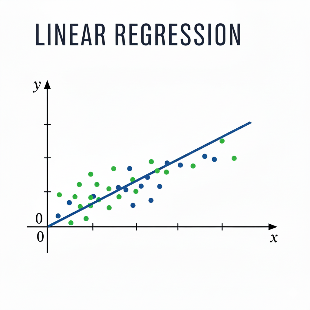
Linear Regression

TL;DR: with a batch of data, find the trend, use the trend to predict, this is linear regression analysis.

For example: 10,000 pieces of data showing the relationship between advertising budget and sales revenue.

The essence of regression analysis is model building and inference(or prediction).
Take above example, the model can tell us what effect it has on revenue for every dollar increase in advertising.
I will use the simplest linear regression to explain.

In order for the model to work properly, we will assume there is some kind of linear relationship between advertising budget and revenue.
Which means, if you spend more money on advertising, revenue will roughly increases.(Not exactly correct, but we assume this trend works)
Besides, we also assume each data point is independent(the sales revenue would not be effected by previous weeks), and model’s prediction error would not get bigger or smaller based on advertising budget.

These assumptions help us to use a simple way to learn how an effective model works.
Of course, reality work would not always follow these assumptions, but we can understand the foundations of a model.

How to build model

1. Mathematic assumption: the purpose of modeling is to find out a formula as close as possible to the trend.
   Take single feature linear regression as example:
   \[ h(x) = w x + b \] We can simplify with:
   \[ \hat{y} = w x + b \] The \(x\) is variable(like advertising budge), \(\hat{y}\) is predicted value(how much revenue gain),
   And \(w_1\)(weight) \(b\)(bias) is the parameters model needs to learn and optimize.

2. Loss Function: measure the error during the training process.
   Based on the error, we can tune the training direction(by changing weight and bias).
   For example, inside the training data, \(x = 1, y = 9\)，
   But the predict value from model is \(x = 1, \hat{y} = 7\), the \(2\) is the error.

   Error = Actual Value - Predicted Value
   9 (Actual Value) - 7(Predicted Value) = Residual

   Error is acceptable, becuz there is no “perfect” model.
   But once an error becomes too big and is classified as an outlier, the function of the Loss Function is precisely to aggregate and utilize. The common way in Loss Function is MSE(Mean Square Error).

3. Optimizer: tune the parameter during the training process By using loss function with proper optimizing strategy to achieve the goal of changing parameter in next iteration.

Loss Function

MSE(Mean Square Error)：
\(J_\mathbf{MSE} = \frac1{m}\sum_{i=1}^{m} (y_{i} - \hat{y}_{i}) ^ 2\)

Q: Why MSE can be use as loss function?

We hope we can find a formula, which can calculates the whole errors during the whole dataset, and we do our best to let this formula as close as possible to zero, which means the performance of model is good.

De-assemble MSE by chart

As you can see from the chart, red line represents the regression line in a training, blue dot is actual value( \(x_i, y_i\) ),x-axis as variable,each dot on the red line is the predicted value( \(\hat{y}\) ) in the given variable x.。
There is some positive error and negative error, the purpose of training is to reduce these error as many as possible.
In the chart, \(\hat{y}_6\) (predicted value)has a huge difference with actual value, we call it outlier, this outlier may cause impact to the training result.

Below it the error base on the chart: \[ \begin{align*} E_i &= y_i - \hat{y}_{i} \\ E_1 &= 50 - 45 = 5 \\ E_2 &= 65 - 55 = 10 \\ E_3 &= 50 - 65 = -15 \\ E_4 &= 90 - 75 = 25 \\ E_5 &= 75 - 85 = -10 \\ E_6 &= 160 - 95 = 65 \end{align*} \] If we are going to calculates the average error, normally way to do it is find average value with summation of errors(Arithmetic Mean):
\[ \frac{1}{m}\sum_{m=1}^{m} E_{i} \] This bring a problem:
Positive and negative error will cancel each other out(or offset), thus we need to find another way to avoid the cancellation.

MAE vs MSE

In match, common way to remove negative value is by take absolute or square. \[ \begin{align*} Mean Absolute Error, MAE &= \frac{1}{m}\sum_{m=1}^{m} \big|E_{i}\big| \\ Mean Square Error, MSE &= \frac{1}{m}\sum_{m=1}^{m} {E_{i}}^2 \end{align*} \] Two ways, which one should we use?
We keep this problem for now, I will answer later.
In the applied math in machine learning, there is no single correct answer; it’s more about trade-offs.

Optimizer

The purpose of optimizing is to gradually change the value of \(w\) in order to reduce the error from loss function, it would be ideal to get zero from loss function.
In machine learning fields, optimizer usually represents gradient-based optimizers,
there is more other optimizing strategy, but we won’t discuss in this article.

Gradient Descent

The essence of a gradient is the derivative, it points to the fastest growth direction at current position(steepest uphill),
In order to make it easier to understand the mathematic theory, I will simplify the predict function \(\hat{y}_i\) into a single-feature function.

Here we let \(b = 0\) is just only to help us to discuss the theory, in practice, you won’t even see this kind of ideal situation. If \(b != 0\) will let the gradient descent function become a dual-feature, that would make this section much more complicated, so I will skip this part here.

\[ \begin{align*} \because Let\space b &= 0 \\ \therefore \hat{y}_i &= wx + 0 \\ &= wx \end{align*} \] We just need to involve with feature \(w\) .

As the chart, this is the relationship between \(w\) weight and \(J(w)\) errors.
I meant to take out all the possibilities of \(w\) to draw the chart, in actual training cases, its more like the system trying-error with each point’s( \(w\) ) value blindly.

As you can see from the chart, when \(w = [11.1, 11.2]\) is inside of this interval, we can find the smallest value of \(J(w)\) .
In mathematics, the way we finding a minimum value of a function is relative with slope.

Slope & Differentiation

By calculate the y-axis’s offset with two dots on a curve, we can get the slope(trend) of these two points.
Take \(w_{best}\) as example, the point that \(J(w)\) is closest to zero(or the minimum of the whole curve) of \(w\) is \(w_{best}\): \[ \begin{align*} J(11.1) &= 581.4066 \\ J(11.2) &= 581.693 \\ m &= (581.693 - 581.4066) / (11.2 - 11.1) \\ &= 0.2864 / 0.1 \\ &= 0.02864 \end{align*} \]

With this slope as tool, it allows us to find out we should increase/decrease the value of \(w\) in order to get minimum \(J(w)\) .
No matter the slope is positive or negative, it always means we need to correct the value in the opposite direction the value of \(w\) in order to get a slope closes zero as many as possible.

In math, to find a slope of any point on a smooth curve, we use differentiation.
\[ \begin{align*} Let\space u &= (y_i - wx_i), f(u) = u ^ 2 \\ J(w) &= \frac{1}{m}\sum_{i=1}^{m}f(u) \\ \dfrac{dJ}{dw} &= \frac{1}{m}\sum_{i=1}^{m}\dfrac{df}{dw} \\ \because \dfrac{df}{dw} &= \dfrac{df}{du} \times \dfrac{du}{dw} \\ &= 2u \times \dfrac{d}{dw}(y_i - wx_i) \\ &= 2u \times (0 - x_i) \\ &= 2(y_i - wx_i) \times -x_i \\ \therefore \dfrac{dJ}{dw} &= \frac{1}{m}\sum_{i=1}^{m}2(y_i - wx_i)(-x_i) \\ &= \frac{2}{m}\sum_{i=1}^{m}(- y_i + wx_i)(x_i) \\ &= \frac{2}{m}\sum_{i=1}^{m}(wx_i - y_i)(x_i) \\ \because \hat{y}_i &= wx_i \\ \therefore \dfrac{dJ}{dw} &= \frac{2}{m}\sum_{i=1}^{m}(\hat{y}_i - y_i)x_i \\ \end{align*} \] Thus, we found the gradient function which can help us make correction on parameter \(w\) created by out loss function.

Optimizing iteration rules

By using gradient formula:\(\dfrac{dJ}{dw} = \frac{2}{m}\sum_{i=1}^{m}(\hat{y}_i - y_i)x_i\)
We can get a optimizer’s iteration rules:\(w_{new} = w_{old} - \alpha \cdot \dfrac{dJ}{dw}\)

Here, \(\alpha\) is a learning rate, works like an amplifying parameter, which controls learning speed and the stability of convergence.

• \(\alpha\) too big: Over-shooting:
  It causes training to jump back and forth near the bottom of the curve, eventually cannot converge
  
• \(\alpha\) too small: Slow Convergence:
  The optimizer will learn in a very slow speed to find the best \(w\) ,but it will be time-consuming.

In actual training \(\alpha\) is called a hyperparameter, it should be setup and manually tuning before training.
We won’t talk about \(\alpha\) here, becuz is comes with much more deep dive, we will skip this part here.

With optimizer in countless training(we called it epochs), \(w\) will move toward the fastest decent direction with curve.
Eventually will let \(J(w)\) became stable, we call it convergence, at this point, the \(w\) is \(w_{best}\).
Then:

\[ \hat{y} = w_{best}x \]

!Massive Calculate! Bonus: Dual-feature gradient descent

Above we let \(b = 0\) in order to make \(\hat{y}\) become single feature, which helps us easier to working on the math.
Now we put back \(b\) : \(\hat{y} = wx + b\)
Then we need to do the partial derivative to \(w\) and \(b\) :
\[ \begin{align*} Define：\\ \hat{y} &= wx + b \\ J(w,b) &= \frac{1}{m}\sum_{i=1}^{m}(y_i - \hat{y}_i) ^ 2 \\ &= \frac{1}{m}\sum_{i=1}^{m}(y_i - (wx_i + b)) ^ 2 \\ Let:\\ u &= (y_i - \hat{y}_i) \\ f(u) &= u ^ 2 \\ \end{align*} \] Then for \(\dfrac{dJ}{dw}\):
\[ \begin{align*} \dfrac{dJ}{dw} &= \frac{1}{m}\sum_{i=1}^{m}\dfrac{df}{dw} \\ \because \dfrac{df}{dw} &= \dfrac{df}{du} \times \dfrac{du}{dw} \\ &= 2u \times \dfrac{d}{dw}(y_i - (wx_i + b)) \\ &= 2u \times (0 - x_i - 0) \\ &= 2u \times - x_i \\ \therefore \dfrac{dJ}{dw} &= \frac{1}{m}\sum_{i=1}^{m} (2u \times - x_i) \\ &= \frac{1}{m}\sum_{i=1}^{m}(2(y_i - \hat{y}_i) \times - x_i) \\ &= \frac{2}{m}\sum_{i=1}^{m}(\hat{y}_i - y_i)x_i \\ \end{align*} \] for \(\dfrac{dJ}{db}\):
\[ \begin{align*} \dfrac{dJ}{db} &= \frac{1}{m}\sum_{i=1}^{m}\dfrac{df}{db} \\ \because \dfrac{df}{db} &= \dfrac{df}{du} \times \dfrac{du}{db} \\ &= 2u \times \dfrac{d}{db}(y_i - (wx_i + b)) \\ &= 2u \times (0 - 0 - 1) \\ &= 2u \times -1 \\ \therefore \dfrac{dJ}{db} &= \frac{1}{m}\sum_{i=1}^{m}(-2u) \\ &= \frac{1}{m}\sum_{i=1}^{m}(-2(y_i - \hat{y}_i)) \\ &= \frac{2}{m}\sum_{i=1}^{m}(\hat{y}_i - y_i) \\ \end{align*} \] Eventually:
\[ \begin{align*} w_{new} &= w_{old} - \alpha \cdot \dfrac{dJ}{dw} \\ &= w_{old} - \alpha \cdot \frac{2}{m}\sum_{i=1}^{m}(\hat{y}_i - y_i)x_i \\ b_{new} &= b_{old} - \alpha \cdot \dfrac{dJ}{db} \\ &= b_{old} - \alpha \cdot \frac{2}{m}\sum_{i=1}^{m}(\hat{y}_i - y_i) \\ \end{align*} \] In the end we can find a simple conclusion:

The correction of \(w\) is affected by \(x_i\); the input of the training data determines the direction of correction.
and the correction of \(b\) is only affected by the mean of total errors, \(b\) only simply moves the whole regression function vertically.

Beside gradient descent?

In math there is still another way called normal equation can calculate the answer of \(w_{best}\) directly,
like OLS(Ordinary least squares), but in machine learning field, its almost not possible with such ideal environment,
Thus in this article, we did not mention such solutions above.

So MAE or MSE?

MAE and MSE are all about collection errors, there is no plain answer to use which of them.
But more about the characteristic of training data and how you want the model performs.

MAE itself, affected by the absolute, the curve would be non-smooth but continuous,
Which is not able to directly find the derivative of whole curve and apply to optimizer’s iteration rules.
It has to use some technique like sub-gradient to deal with the non-differentiable point.
In practice there is something more to do with optimizer, we will skip this part here.

Last

This article discusses the simplest linear regression with MSE in machine learning field and its mathematic theory.
The field of machine learning is vast. I wrote this article as a way to prepare for the AWS AI Practitioner(AIF-C01) and to figure out some parts I didn’t fully understand before. It also helped me to brush up on my Calculus(or rescue my falling Calculus knowledge)…